Linear Discriminant Analysis
Linear Discriminant Analysis is an algorithm the goal of which is the same as Principal Component Analysis: reducing the dimension of your dataset. However, this algorithm doesn't try to find out the important parameters, but to find a simple form to represent your many patients clearly separated in categories based on the information it's given, which would usually take a much more complex graphic representation.
How does it work?
This algorithm seeks to find an axis along which the types of patients are clearly separated and classified, and it does so by maximizing the distance between the central points of each type of patient (their means), while minimizing how scattered (spread out) the patients are along this new axis.
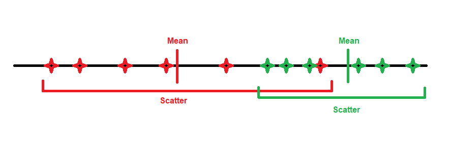
The process begins by taking the info we have on patients and classifying it in groups, that we will call classes. Then, we distribute them on a space of as many dimensions as variables we have. For the sake of understanding, we'll work with 2 dimensions: height and weight, so we distribute our patients in a plane.
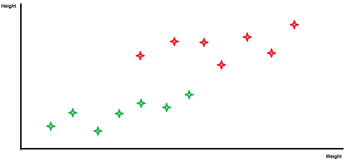
Now, the algorithm will find the central point of each of our classes (its mean), and measure the distance between them. It is as important to maximize the distance between means as it is to minimize the scattering, because only doing both we guarantee that there's the optimal separation of groups.
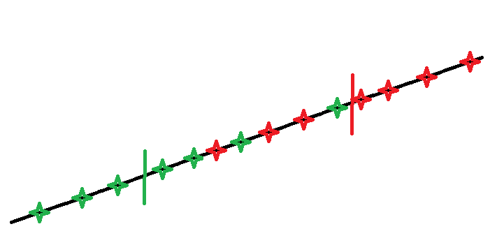
In this case, we're only trying to maximize the distance between means, but as you can see, there's a little bit of a mix-up between the two classes.
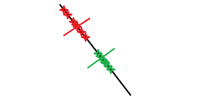
However, here we're trying to minimize the scattering as well. Even though the distance between means is not as big as before, there's a much more clear separation between class A and class B.
An example
For better understanding, let's imagine we're doing a study where we test a drug related to breathing issues during the night on 15 patients. After we've done some testing, we realise that there's essentially 3 groups of patients: Patients who react positively to the drug, patients who react negatively, and patients who just don't feel any different. We will have, therefore, 3 classes. We will suppose that in this study we take into account the weight and the height of our participants. When we spread them out in a graph, this is the result.
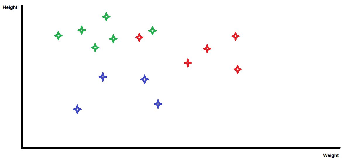
Red dots represent patients with negative reactions, green dots represent the ones with positive reactions and blue dots are patients who felt the same.
In this example, we will not be able to do the same as before and collapse everything into 1 dimension, since we have 3 classes and this will change a few things. First of all, we will need 2 axes to separate all 3 categories of patients. If we tried to do it all in 1 axis, the classes would intertwine and end up being poorly classified. Also, we will need to find the center point of all the data, and we will calculate the distance between the mean of every class and said point, instead of calculating the distance between two means. It will result in something along the lines of the following image.
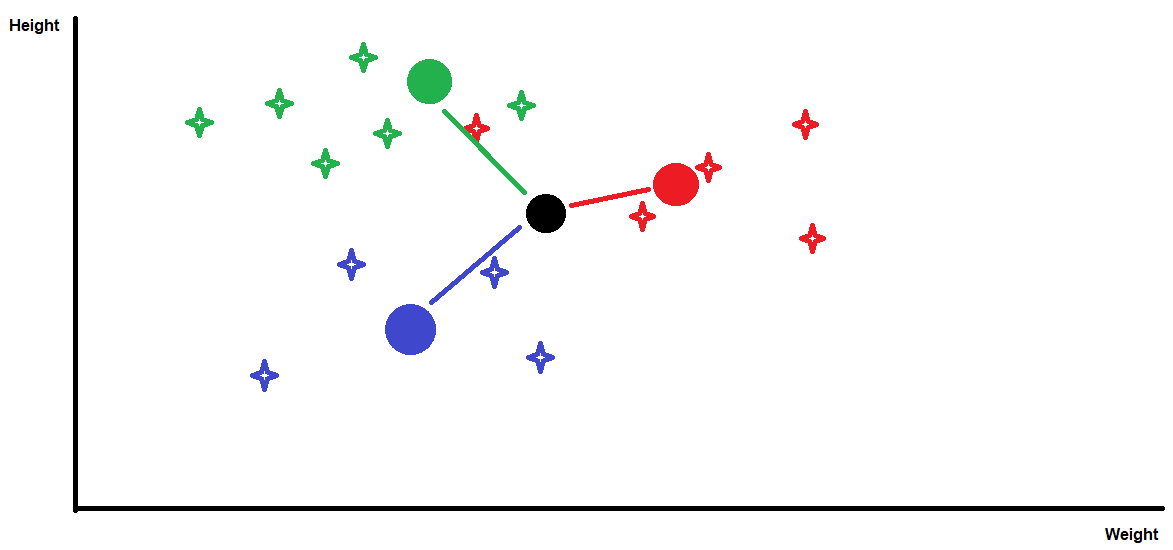
Now, the algorithm will try to maximize the distance between the means, just as before, and minimize the scatter of each group. This way, we will have the 3 classes clearly separated and classified. Even though this example is applied to only 3 classes and 2 variables, and therefore the dimensionality reduction is not there (we go from a 2D graph to another 2D graph), the algorithm would work through the same steps if we had a thousand different variables, as is usual in this kind of test, and would result in a considerable reduction of the dimensionality of our data.
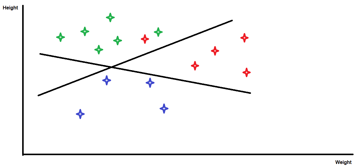
As we see, the classification isn't perfect, but it still gives us quite an accurate idea of which patients will feel better by taking the drug based on their height and weight.